Abstract
carnation is an interactive Shiny dashboard that
simplifies and transforms complex bulk RNA-Seq and multi-omic data
using insightful visualizations and numerous interactive features.
Designed for both computational and experimental biologists,
carnation unifies three facets of differential
expression analysis, functional enrichment, and pattern analysis
making data exploration intuitive and accessible, while also
providing a platform to manage multiple datasets either locally or
on a server to share with collaborators (package version:
1.1.0).
Now, we will use the airway dataset to explore some of
carnation's functionality.
Install carnation
Install carnation from Bioconductor using
BiocManager::install.
# first check to see if BiocManager is available
if(!requireNamespace('BiocManager', quietly=TRUE)){
  install.packages('BiocManager')
}

BiocManager::install('carnation')
Load libraries & airway dataset
First check for and load some libraries that we will need for this tutorial.
# install optional packages if not present
pkgs_to_check <- c('airway', 'org.Hs.eg.db', 'DEGreport')
for(pkg in pkgs_to_check){
  if(!requireNamespace(pkg, quietly=TRUE)){
    BiocManager::install(pkg)
  }
}We will be using the ‘airway’ dataset. First, we load this dataset.
data('airway')Next, we extract the counts matrix and and metadata.
Now let’s see what these look like.
dim(mat)
#> [1] 63677     8
So, mat is a matrix with 64102 rows and 8 columns. Each
row corresponds to a single gene and each column corresponds to a single
sample. As you will notice, the rownames of mat contains
gene IDs and column names have the sample IDs.
head(mat)
#>                 SRR1039508 SRR1039509 SRR1039512 SRR1039513 SRR1039516
#> ENSG00000000003        679        448        873        408       1138
#> ENSG00000000005          0          0          0          0          0
#> ENSG00000000419        467        515        621        365        587
#> ENSG00000000457        260        211        263        164        245
#> ENSG00000000460         60         55         40         35         78
#> ENSG00000000938          0          0          2          0          1
#>                 SRR1039517 SRR1039520 SRR1039521
#> ENSG00000000003       1047        770        572
#> ENSG00000000005          0          0          0
#> ENSG00000000419        799        417        508
#> ENSG00000000457        331        233        229
#> ENSG00000000460         63         76         60
#> ENSG00000000938          0          0          0
cdata contains the sample metadata. There is a lot of
information here, but notice the cell and dex
columns, as we will be using this for the differential expression
analysis later.
cdata
#> DataFrame with 8 rows and 9 columns
#>            SampleName     cell      dex    albut        Run avgLength
#>              <factor> <factor> <factor> <factor>   <factor> <integer>
#> SRR1039508 GSM1275862  N61311     untrt    untrt SRR1039508       126
#> SRR1039509 GSM1275863  N61311     trt      untrt SRR1039509       126
#> SRR1039512 GSM1275866  N052611    untrt    untrt SRR1039512       126
#> SRR1039513 GSM1275867  N052611    trt      untrt SRR1039513        87
#> SRR1039516 GSM1275870  N080611    untrt    untrt SRR1039516       120
#> SRR1039517 GSM1275871  N080611    trt      untrt SRR1039517       126
#> SRR1039520 GSM1275874  N061011    untrt    untrt SRR1039520       101
#> SRR1039521 GSM1275875  N061011    trt      untrt SRR1039521        98
#>            Experiment    Sample    BioSample
#>              <factor>  <factor>     <factor>
#> SRR1039508  SRX384345 SRS508568 SAMN02422669
#> SRR1039509  SRX384346 SRS508567 SAMN02422675
#> SRR1039512  SRX384349 SRS508571 SAMN02422678
#> SRR1039513  SRX384350 SRS508572 SAMN02422670
#> SRR1039516  SRX384353 SRS508575 SAMN02422682
#> SRR1039517  SRX384354 SRS508576 SAMN02422673
#> SRR1039520  SRX384357 SRS508579 SAMN02422683
#> SRR1039521  SRX384358 SRS508580 SAMN02422677
Get more gene annotation
The gene IDs that come with the dataset are from ENSEMBL and are not
human-readable. So, next we will extract gene symbols and
ENTREZID for these genes from the org.Hs.eg.db
package.
keytypes <- list('SYMBOL'='SYMBOL', 'ENTREZID'='ENTREZID')

anno_df <- do.call('cbind',
             lapply(keytypes, function(x){
               mapIds(org.Hs.eg.db,
                 column=x,
                 keys=rownames(mat),
                 keytype='ENSEMBL')
               })
             )

# convert to data frame
anno_df <- as.data.frame(anno_df)
Now, we have human readable gene names in the SYMBOL
column and Entrez IDs in the ENTREZ column.
head(anno_df)
#>                 SYMBOL ENTREZID
#> ENSG00000000003 TSPAN6     7105
#> ENSG00000000005   TNMD    64102
#> ENSG00000000419   DPM1     8813
#> ENSG00000000457  SCYL3    57147
#> ENSG00000000460  FIRRM    55732
#> ENSG00000000938    FGR     2268
Create DESeqDataSet
Next, we create a new DESeqDataSet using
mat and cdata.
dds <- DESeqDataSetFromMatrix(mat,
                              colData=cdata,
                              design=~cell + dex)
Let’s check to make sure that everything looks okay:
dds
#> class: DESeqDataSet
#> dim: 63677 8
#> metadata(1): version
#> assays(1): counts
#> rownames(63677): ENSG00000000003 ENSG00000000005 ... ENSG00000273492
#>   ENSG00000273493
#> rowData names(0):
#> colnames(8): SRR1039508 SRR1039509 ... SRR1039520 SRR1039521
#> colData names(9): SampleName cell ... Sample BioSample
Then we save dds in a list.
dds_list <- list(main=dds)We also normalize the counts data and save it in a list.
rld_list <- lapply(dds_list, function(x) varianceStabilizingTransformation(x, blind=TRUE))Run differential expression analysis
Now, the object dds is ready for differential expression
(DE) analysis.
dds <- DESeq(dds)
#> estimating size factors
#> estimating dispersions
#> gene-wise dispersion estimates
#> mean-dispersion relationship
#> final dispersion estimates
#> fitting model and testing
Since, we used design=~cell + dex while creating
dds, the above step will automatically calculate some
comparisons.
resultsNames(dds)
#> [1] "Intercept"               "cell_N061011_vs_N052611"
#> [3] "cell_N080611_vs_N052611" "cell_N61311_vs_N052611"
#> [5] "dex_untrt_vs_trt"
The last comparison dex_untrt_vs_trt contains the effect
of the dex treatment, while the other comparisons compare
different cell lines. Next, we will extract two of these results and run
lfcShrink on them.
For the cell comparison, we choose a precomputed results
using the coef parameter.
cell_comparison <- lfcShrink(dds,
                             coef='cell_N61311_vs_N052611',
                             type='normal')
For the dex comparison, we use contrast to
specify the direction of the comparison, since we want to use
untrt as control.
Now, each of these comparisons, contain the DE analysis results. For example,
head(dex_comparison)
#> log2 fold change (MAP): dex trt vs untrt
#> Wald test p-value: dex trt vs untrt
#> DataFrame with 6 rows and 6 columns
#>                   baseMean log2FoldChange     lfcSE      stat      pvalue
#>                  <numeric>      <numeric> <numeric> <numeric>   <numeric>
#> ENSG00000000003 708.602170     -0.3741527 0.0988429 -3.787752 0.000152016
#> ENSG00000000005   0.000000             NA        NA        NA          NA
#> ENSG00000000419 520.297901      0.2020620 0.1097395  1.842943 0.065337292
#> ENSG00000000457 237.163037      0.0361672 0.1383377  0.264356 0.791505742
#> ENSG00000000460  57.932633     -0.0844567 0.2498904 -0.307054 0.758801924
#> ENSG00000000938   0.318098     -0.0841390 0.1513343 -0.393793 0.693733530
#>                       padj
#>                  <numeric>
#> ENSG00000000003 0.00128292
#> ENSG00000000005         NA
#> ENSG00000000419 0.19646985
#> ENSG00000000457 0.91141962
#> ENSG00000000460 0.89500478
#> ENSG00000000938         NA
Then, we save these results in a special nested list that
carnation will use. Here,
-
rescontains the actual DE analysis results -
ddscontains the name of the DESeqDataSet used for the DE analysis. These values should map todds_listnames -
labelis a description of the comparison
res_list <- list(
        dex_trt_vs_untrt=list(
            res=dex_comparison,
            dds='main',
            label='dex, treated vs untreated'),
        cell_N61311_vs_N052611=list(
            res=cell_comparison,
            dds='main',
            label='cell, N61311 vs N052611')
        )
Finally, we add SYMBOL and ENTREZID columns
to the DE results from the anno_df data frame.
Add functional enrichment results (optional)
Now we run functional enrichment on the DE genes from the two comparisons. For this, we first set significance thresholds and then extract the DE genes and save as a list.
# padj cutoff
alpha <- 0.01

# log2FoldChange threshold; 1 == 2x difference
lfc_threshold <- 1

# list to save DE genes
de.genes <- lapply(res_list, function(x){
              # changed genes
              idx <- x$res$padj < alpha &
                     !is.na(x$res$padj) &
                     abs(x$res$log2FoldChange) >= lfc_threshold

              # return DE genes as a dataframe
              x$res[idx, c('gene', 'ENTREZID')]
            })
Next, we run functional enrichment and save the results in a list
called enrich_list. We also save a converted list called
genetonic which carnation uses for several plots from the
GeneTonic package.
Since, this is a time-consuming step, we will use the pre-computed enrichment results included with carnation.
# fe results from dex comparison
data(eres_dex, package='carnation')

# fe results from dex comparison
data(eres_cell, package='carnation')

# compile into a list
go_list <- list(dex_trt_vs_untrt=eres_dex, cell_N61311_vs_N052611=eres_cell)

# list to save functional enrichment results
enrich_list <- list()

# list to save a converted object for GeneTonic plots
genetonic <- list()

for(comp in names(res_list)){
    # NOTE: this is the command used to generate the functional
    # enrichment results
    #go.res <- clusterProfiler::enrichGO(
    #        gene=de.genes[[comp]][['ENTREZID']],
    #        keyType='ENTREZID',
    #        OrgDb=org.Hs.eg.db,
    #        ont='BP',
    #        pvalueCutoff=1, qvalueCutoff=1,
    #        readable = TRUE)

    # we use the precomputed results here instead
    go.res <- go_list[[ comp ]]

    enrich_list[[ comp ]] <- list(
                               res=comp,
                               changed=list( BP=as.data.frame(go.res) )
                             )

    genetonic[[ comp ]] <- list(
                             res=comp,
                             changed=list(
                               BP=carnation::enrich_to_genetonic(go.res, res_list[[comp]]$res)
                             )
                           )

}
#> Found 2483 gene sets in `enrichResult` object, of which 2483 are significant.
#> Converting for usage in GeneTonic...
#> Found 3706 gene sets in `enrichResult` object, of which 3706 are significant.
#> Converting for usage in GeneTonic...
enrich_list is a nested list where:
- The top-level names are unique keys/identifiers
- The second level corresponds to direction of change,
e.g.
up,downorchanged. This level also contains a special entryreswhich maps tores_listnames, as a way to record where the DE results came from. - The third level corresponds to the ontology, e.g.
BP(GO Biological Process).
Here, we are just using changed genes and the GO Biological Process
(BP) ontology, so enrich_list looks like:
enrich_list
  ├─ dex_trt_vs_untrt
  │    ├─ res = 'des_trt_vs_untrt'    <--- comparison used to get FE results
  │    └─ changed
  │         └─ BP                     <--- functional enrichment results
  │
  └─ cell_N61311_vs_N052611
       ├─ res = 'cell_N61311_vs_N052611'    <--- comparison used to get FE results
       └─ changed
            └─ BP                           <--- functional enrichment results
genetonic mirrors the same structure.
Add pattern analysis (optional)
Finally, we add some pattern analysis for the
dex_trt_vs_untrt comparison using the
DEGreport package. First, we extract normalized data for
the 755 DE genes from this comparison.
# extract normalized data & metadata
ma <- assay(rld_list[['main']])
colData.i <- colData(rld_list[['main']])

# only keep data from DE genes
idx <- rownames(ma) %in% de.genes[['dex_trt_vs_untrt']][['gene']]
ma.i <- ma[idx,]

# remove any genes with 0 variance
ma.i <- ma.i[rowVars(ma.i) != 0, ]
Then, we run the pattern analysis, using cell as the
time variable and dex as the color
variable.
Again, since this is a time-consuming step, we will use the pre-computed pattern analysis results included with carnation.
# NOTE: This is the command used to perform pattern analysis
# degpatterns_dex <- DEGreport::degPatterns(
#                      ma.i,
#                      colData.i,
#
#                      time='cell',
#                      col='dex',
#
#                      # NOTE: reduce and merge cutoff----------------------------------------
#                      #   Reduce will merge clusters that are similar; similarity determined
#                      #   by cutoff
#                      reduce=TRUE,
#
#                      plot=FALSE
#                    )

# We use the pre-computed results here instead
data(degpatterns_dex, package='carnation')
Next, we extract the normalized slot from this object
and save as a list.
# extract normalized slot and add symbol column
p_norm <- degpatterns_dex$normalized
p_norm[[ 'SYMBOL' ]] <- anno_df[p_norm[['genes']], 'SYMBOL']

# save pattern analysis results
degpatterns <- list(dex_by_cell=p_norm)Data Organization
Organize your data in a directory structure that Carnation can easily
navigate, e.g. in a folder carnation/data in your home
directory. Here, we make a subfolder airway in this folder
and copy the RDS file we created above.
~/carnation/data/
  └─ airway
     └─ carnation-vignette.rds
Now, we’re ready for the first run.
First Run
Load the carnation package.
library(carnation)
#>
#> Attaching package: 'carnation'
#> The following object is masked from 'package:GeneTonic':
#>
#>     gs_radar
Carnation allows you to download interactive plots as PDF. To use this functionality you need to install some required Python dependencies:
install_carnation() # Installs plotly and kaleido for PDF exportNow, run the app:
To run on a fixed port, e.g. when using remote servers with SSH port
forwarding, specify port within a list of options.
run_carnation(options=list(port=12345, launch.browser=FALSE))Then access Carnation by opening the URL:
http://127.0.0.1:12345
Initial setup
-
The first time you run carnation, you will be asked to specify where your data is located with a modal dialog.
Enter the folder where you saved the RDS file,
~/carnation/data, then click ‘OK’.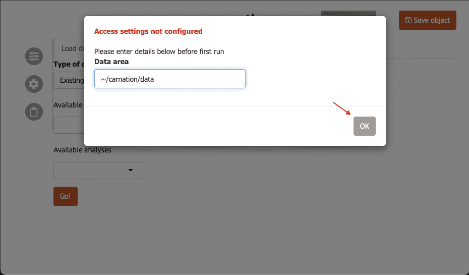
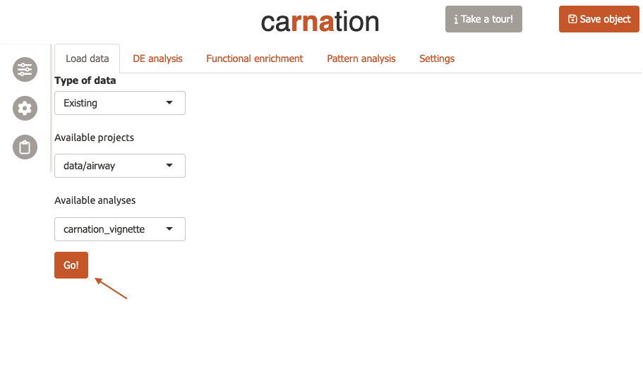
-
Now carnation will automatically refresh and you will see
data/airwayin the “Available Projects” menu, andcarnation_vignettein the “Available Datasets”.On the right, you will see a table summarizing the projects available to carnation. Since this is the only dataset we have, these options are automatically selected. Now click ‘Go’ to load the data.
Now carnation will load the airway data and switch to the “Summary” tab.
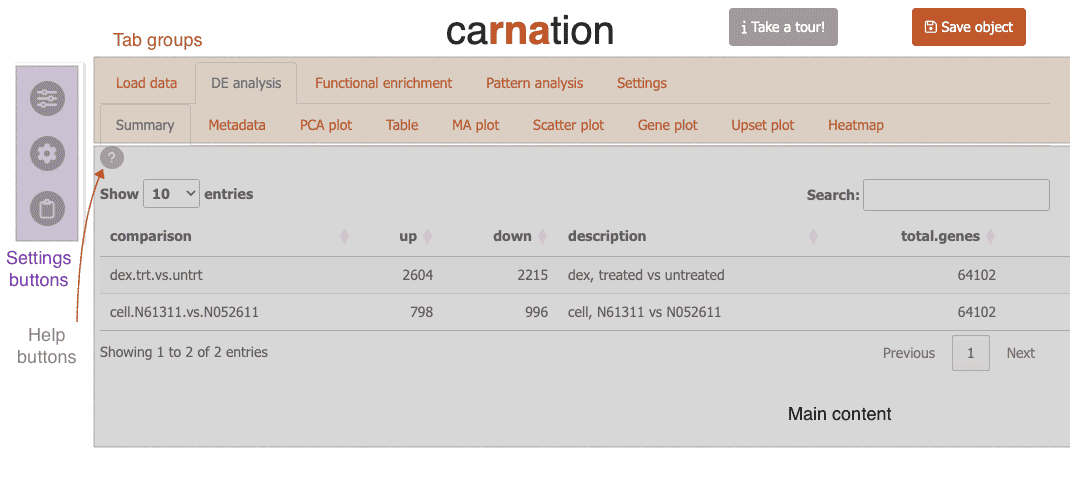
Feature overview
Carnation is organized into three major sections each with its own set of subtabs to organize different portions of the RNA-Seq analysis.
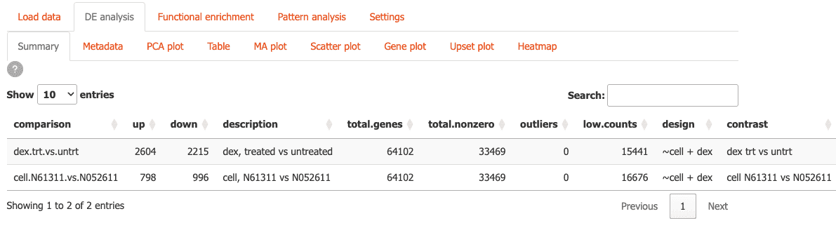
DE analysis
Here you can analyze differential expression through different tables and visualizations:
-
Summary: Get a quick overview of your differential expression results
-
Metadata: Explore sample metadata and experimental design. You can also add metadata columns.
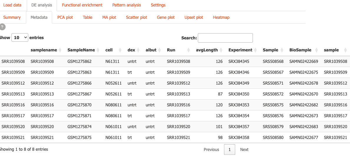
-
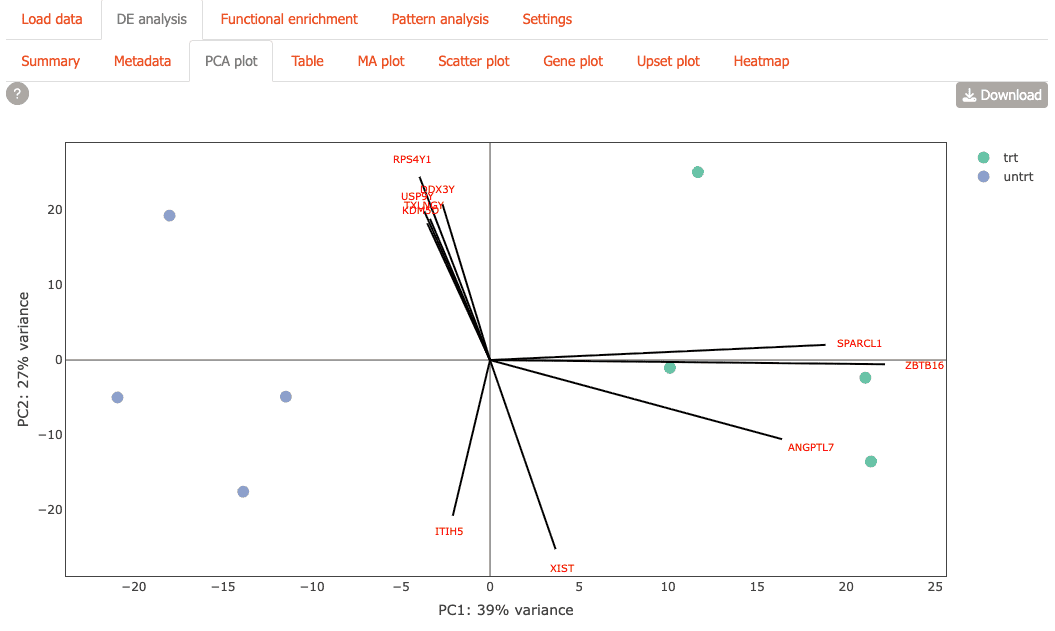
PCA Plot: Visualize sample relationships with PCA plot.
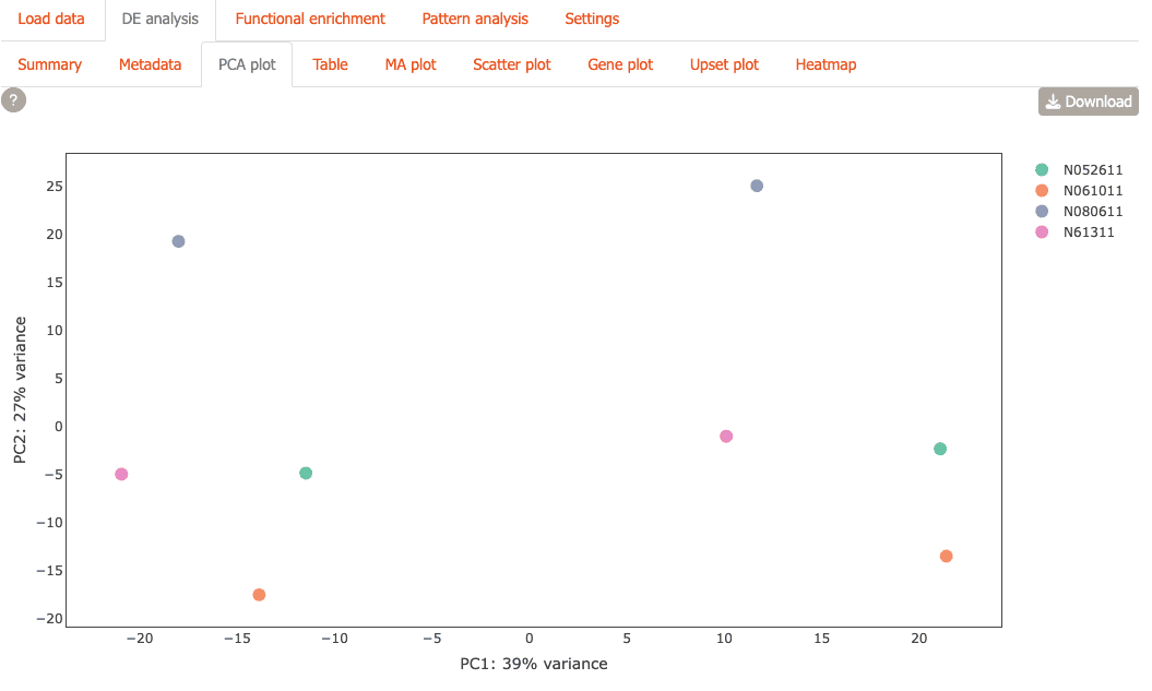
You can also view the plot in 3D
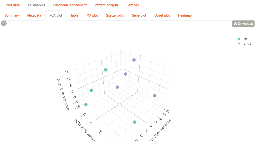
or with gene loadings overlaid.
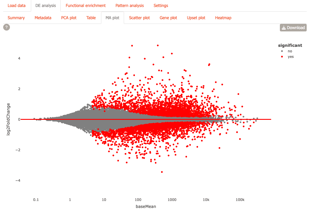
-
MA Plot: Identify differentially expressed genes with statistical significance
-
Scatter Plot: Compare fold-changes of genes across different comparisons

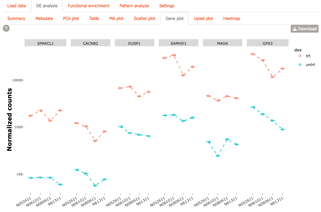
-
Gene Plot: Create customizable expression visualizations for genes of interest
-
UpSet Plot: Discover overlapping gene sets across multiple comparisons

-
Heatmap: Examine expression patterns across samples and conditions

Functional enrichment
Explore functional enrichment analysis results using this module:
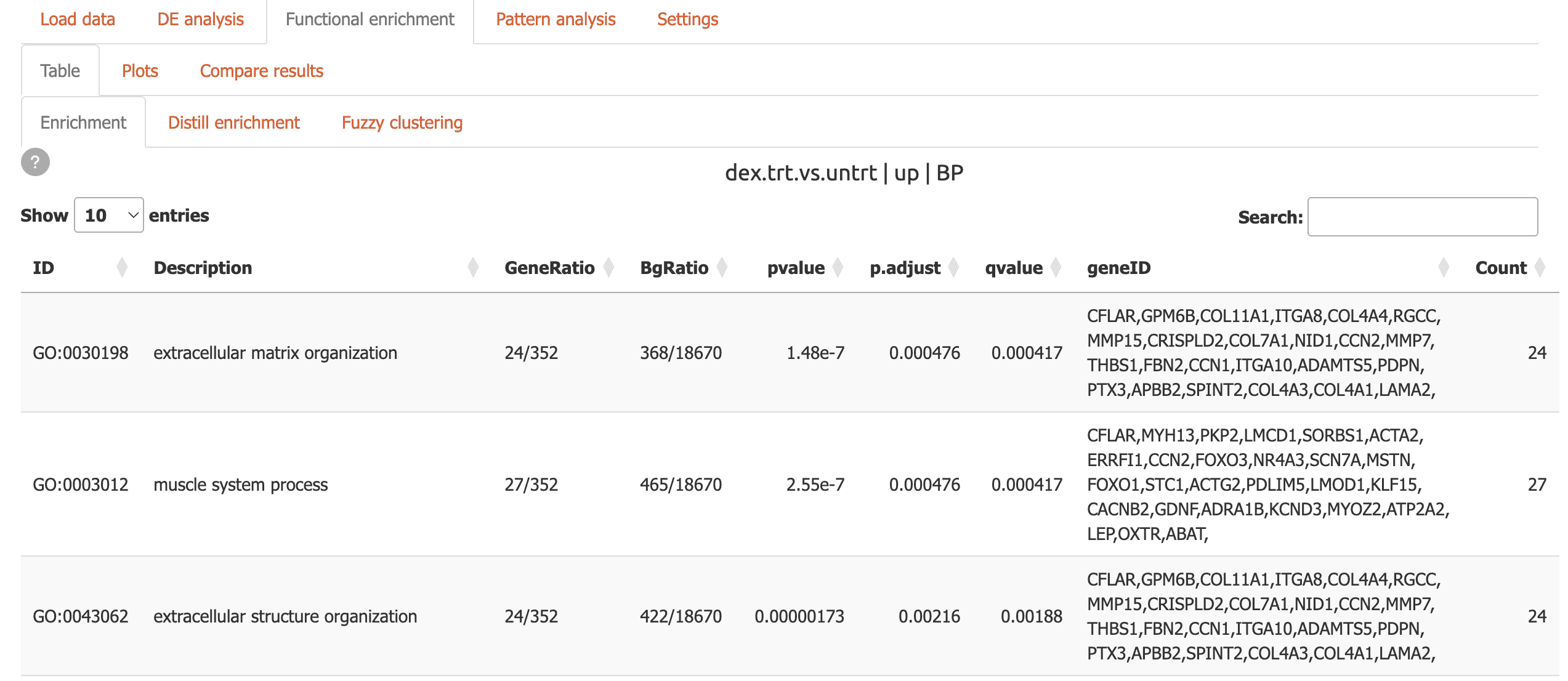
-
Table: Interactive tables with powerful search capabilities
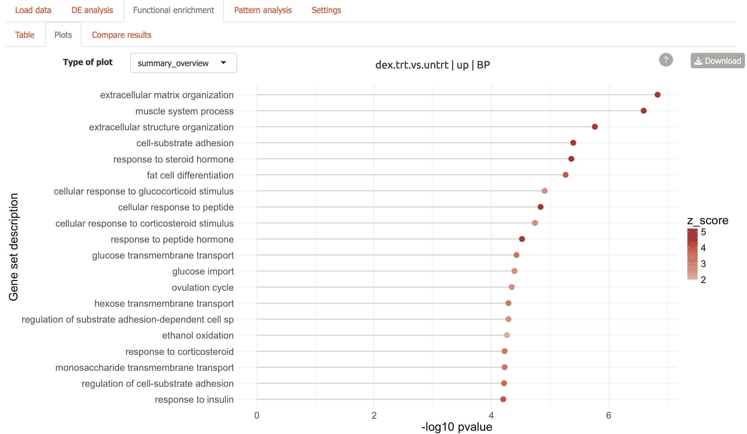
-
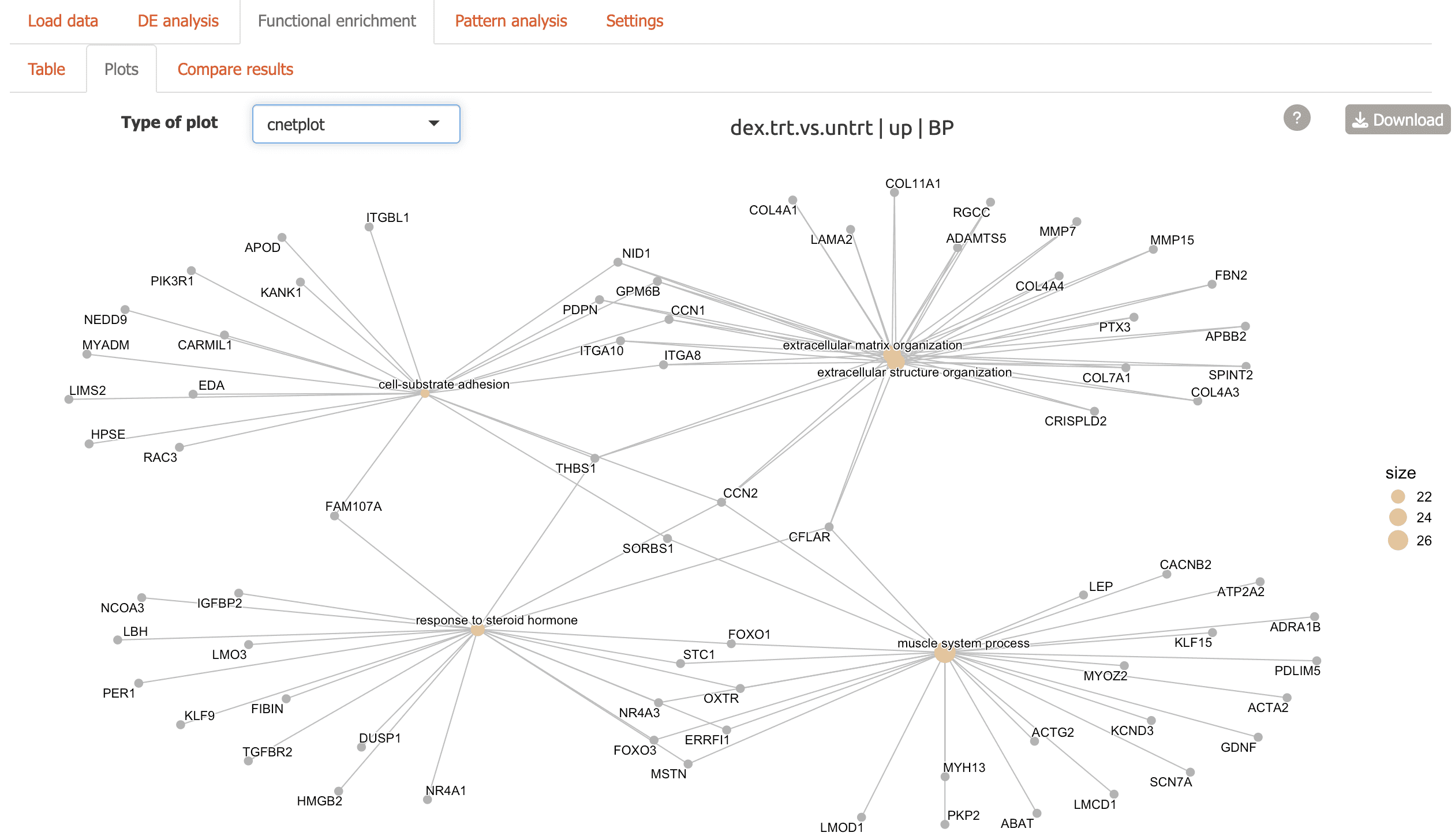
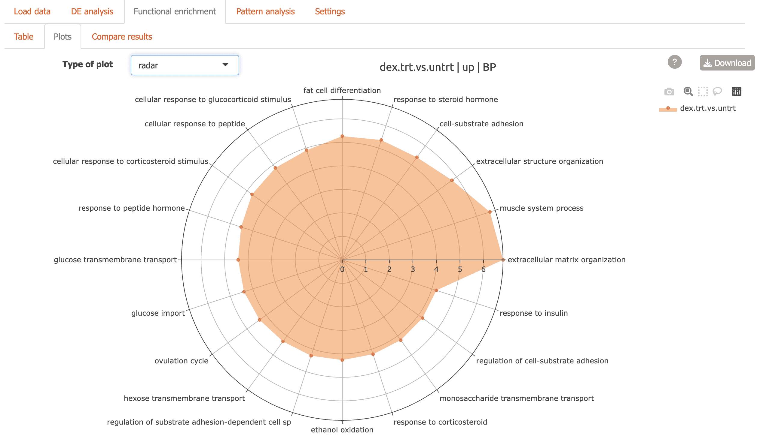
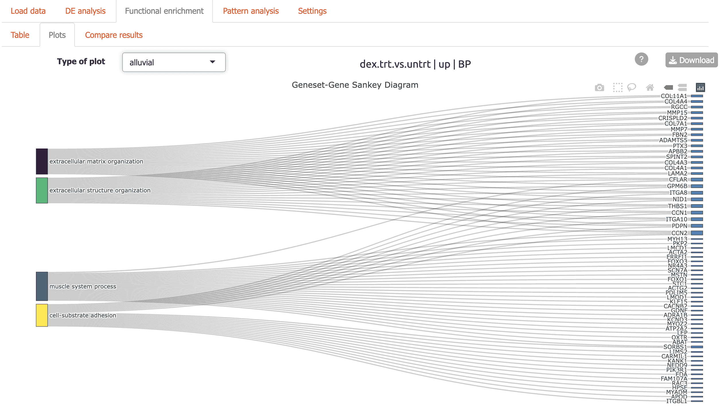
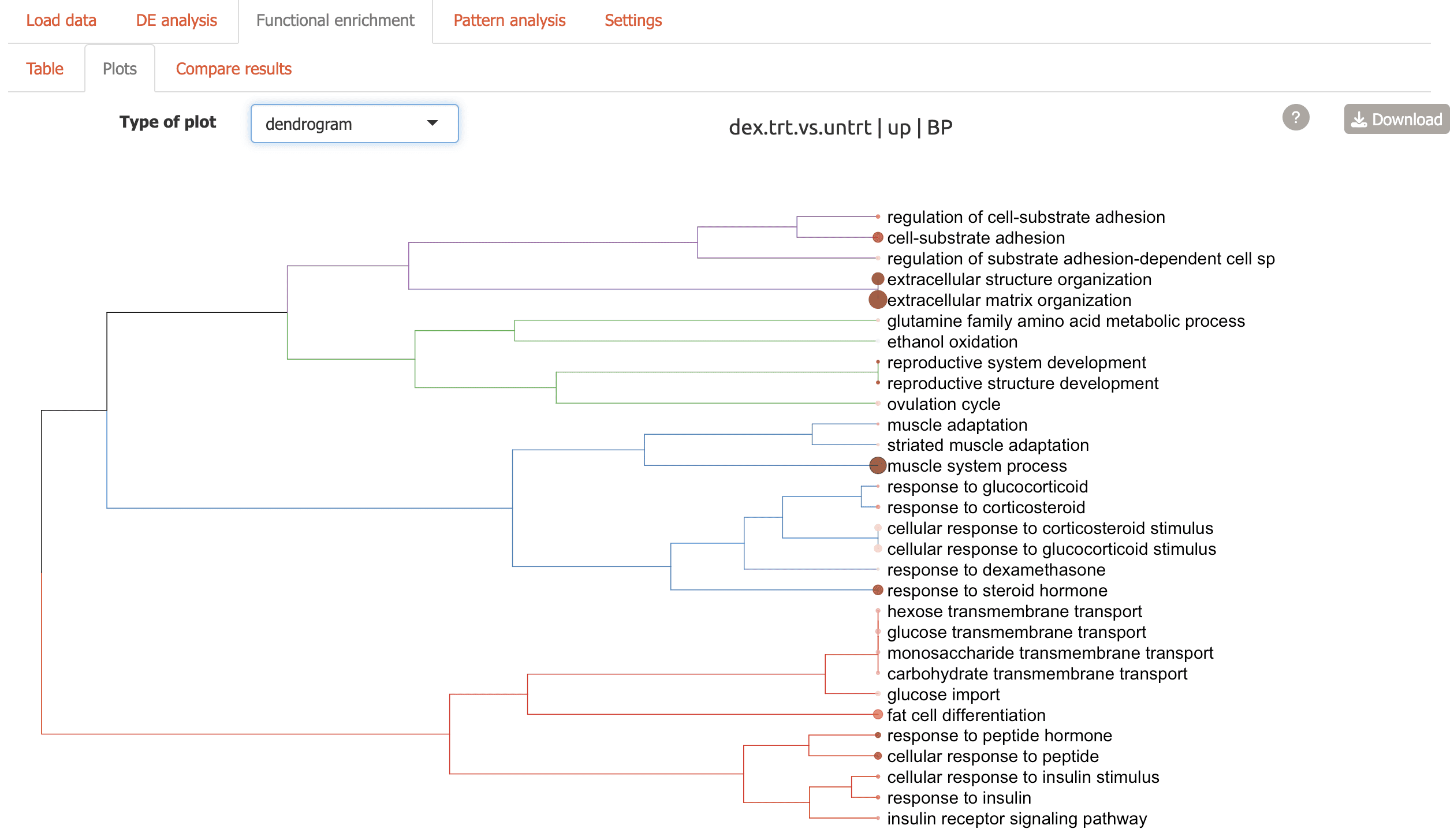
Plots: Seven different visualizations including network plots and dendrograms from the GeneTonic and clusterProfiler packages:
Summary overview to view top enriched terms
Three flavors of enrichment map including one with similar terms grouped together
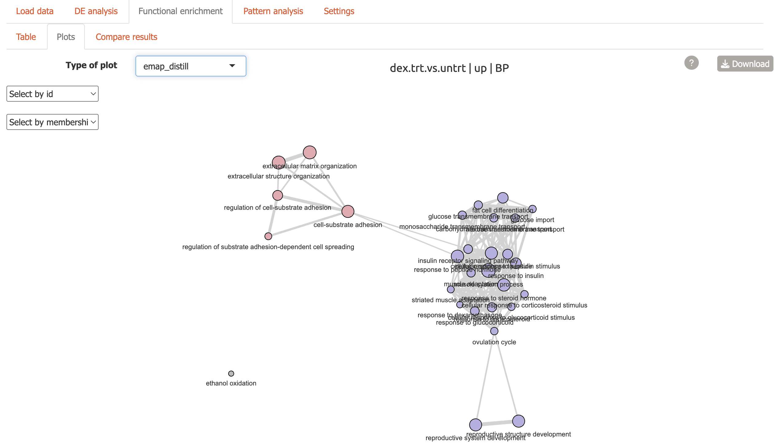
Cnetplot: network plot highlighting genes connecting functional terms
Radar plot: top enriched terms shown in a circular view
Alluvial plot: flow diagram highlighting genes connecting functional terms
Dendrogram: hierarchical tree view of top enriched terms
-
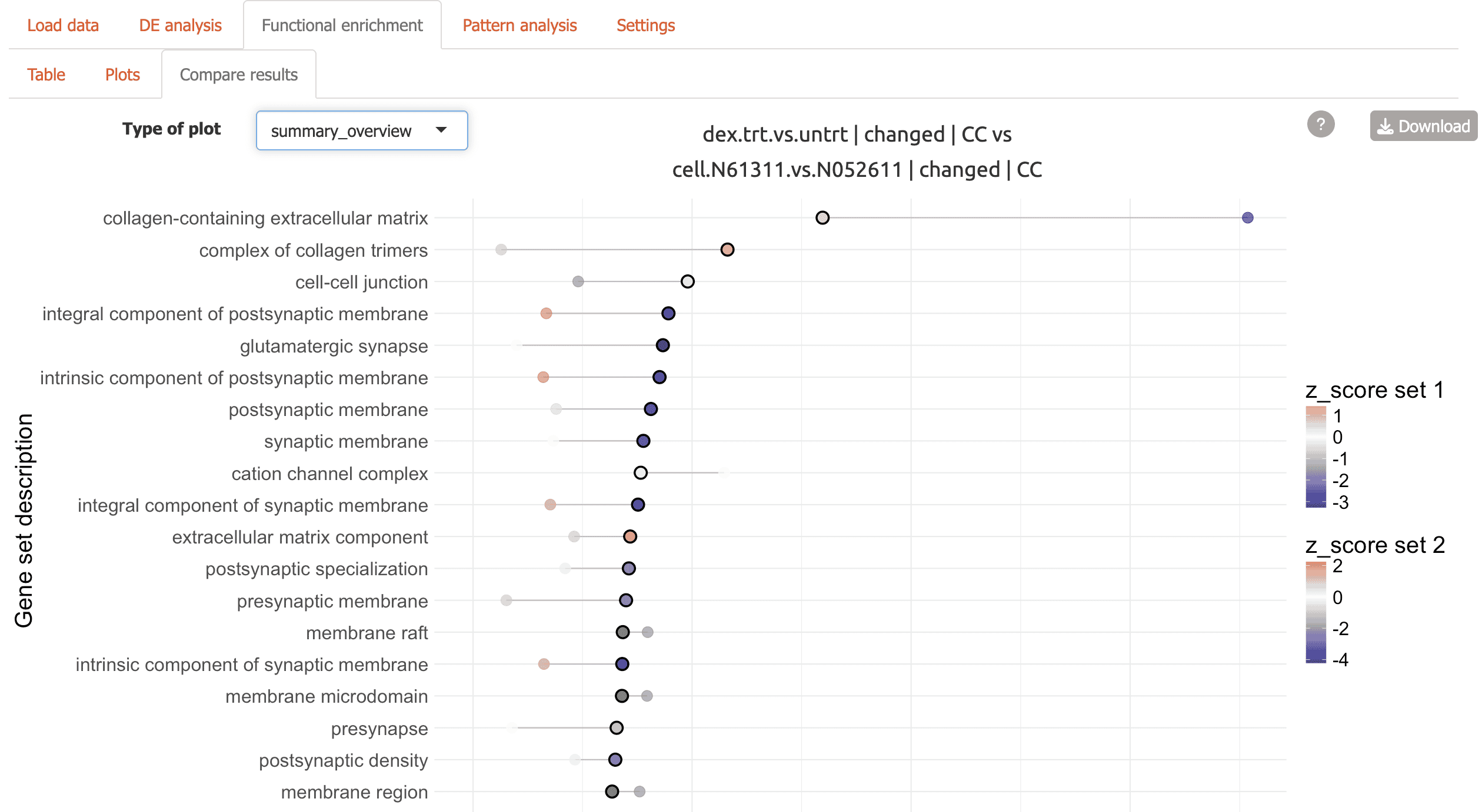
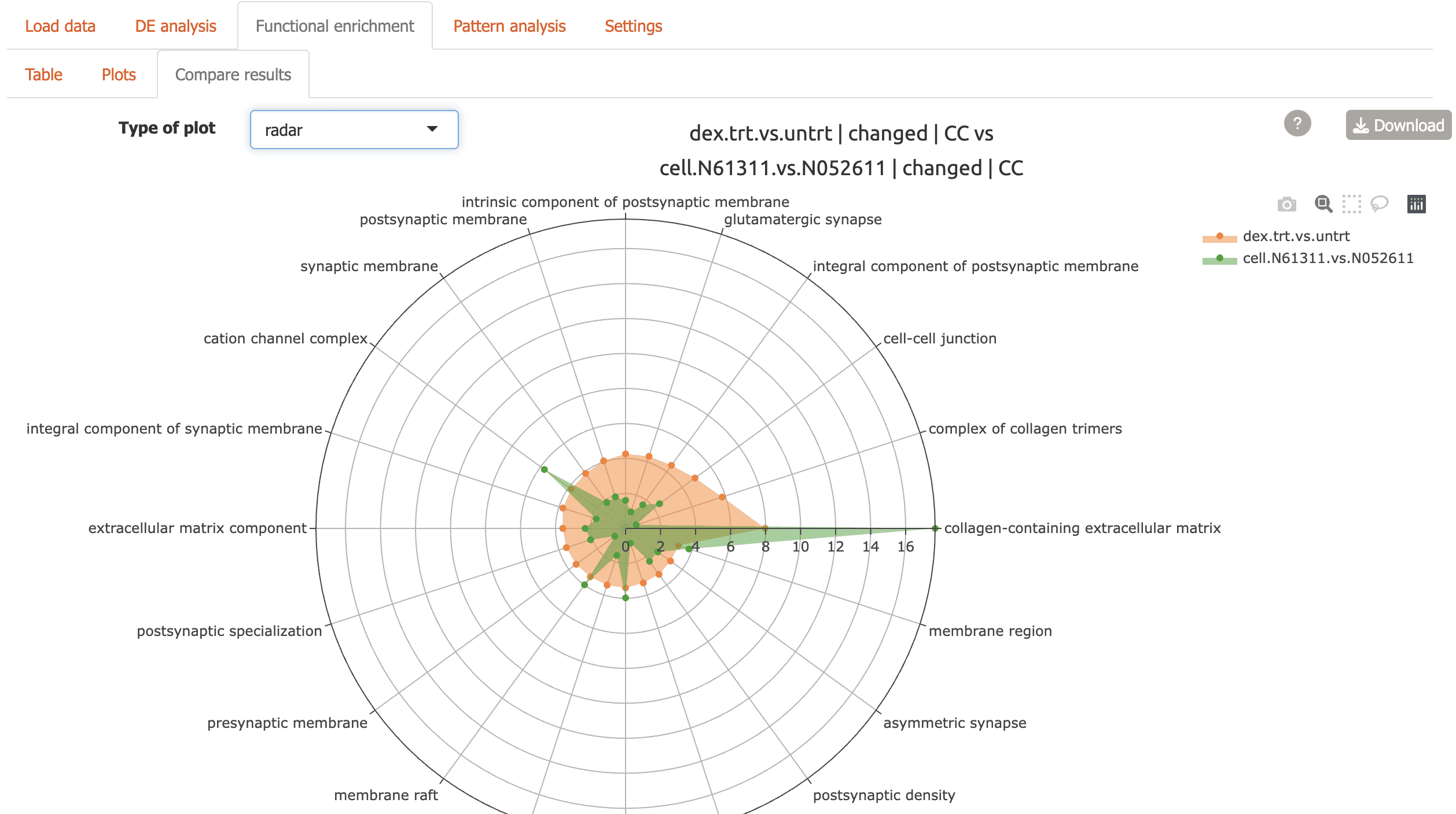
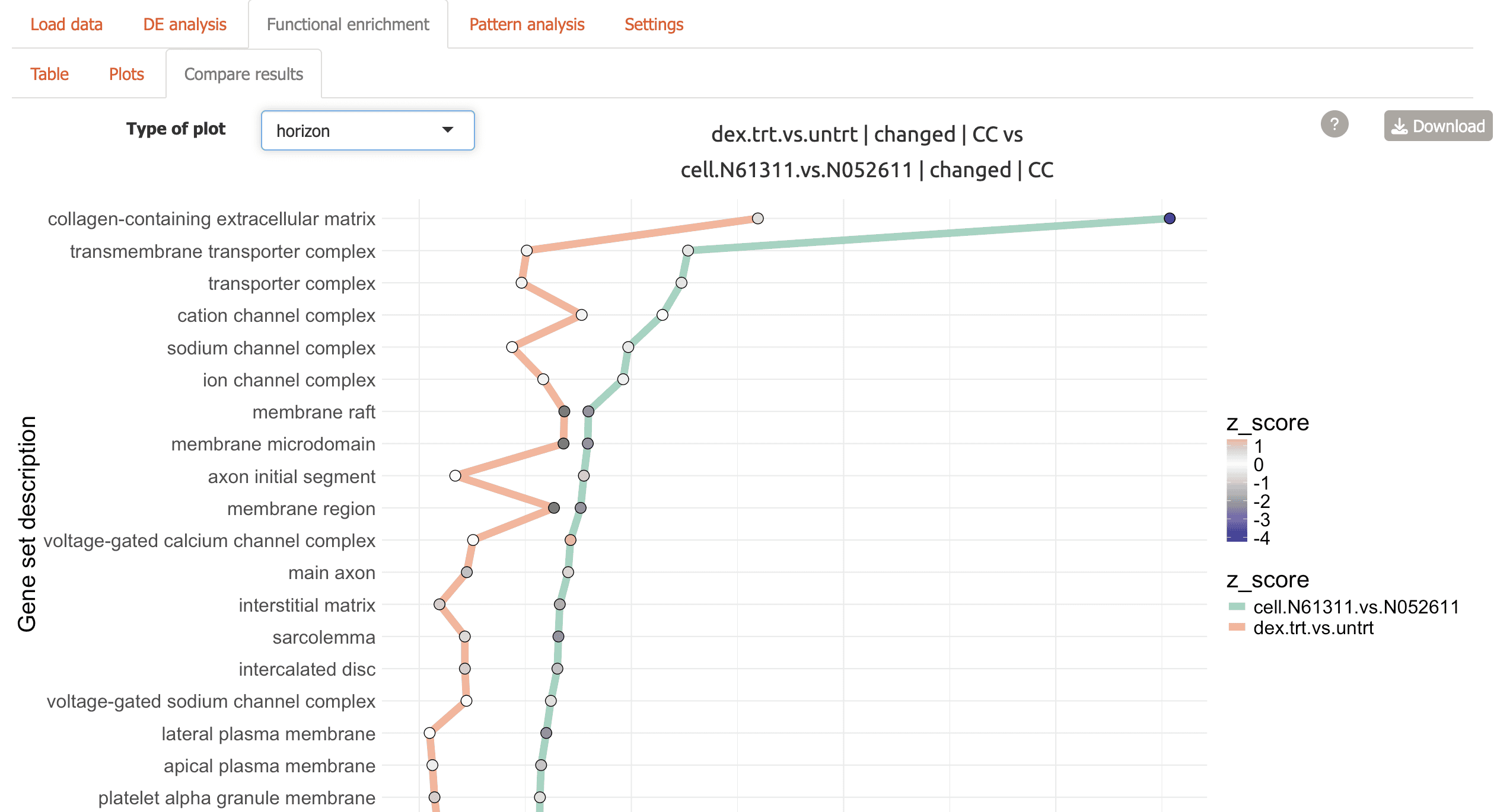
Compare Results: Directly compare enrichment results between conditions using three different visualizations.
Summary overview comparing contrasts
-
Radar plot for two comparisons
Horizon plot for top terms connected by comparison
Pattern analysis
Identify co-regulated gene clusters across conditions
- Plot: Visualize expression patterns of gene clusters
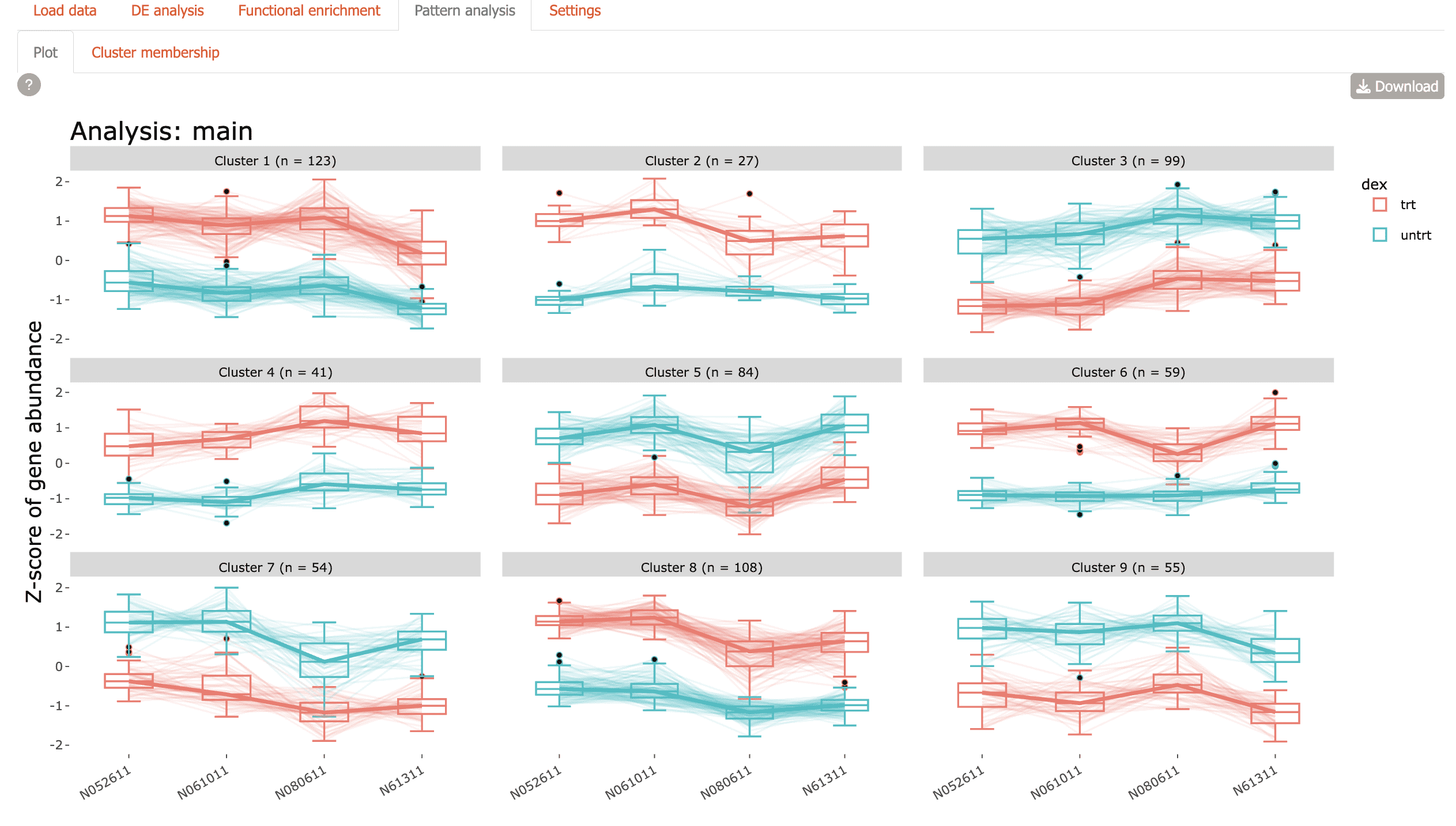
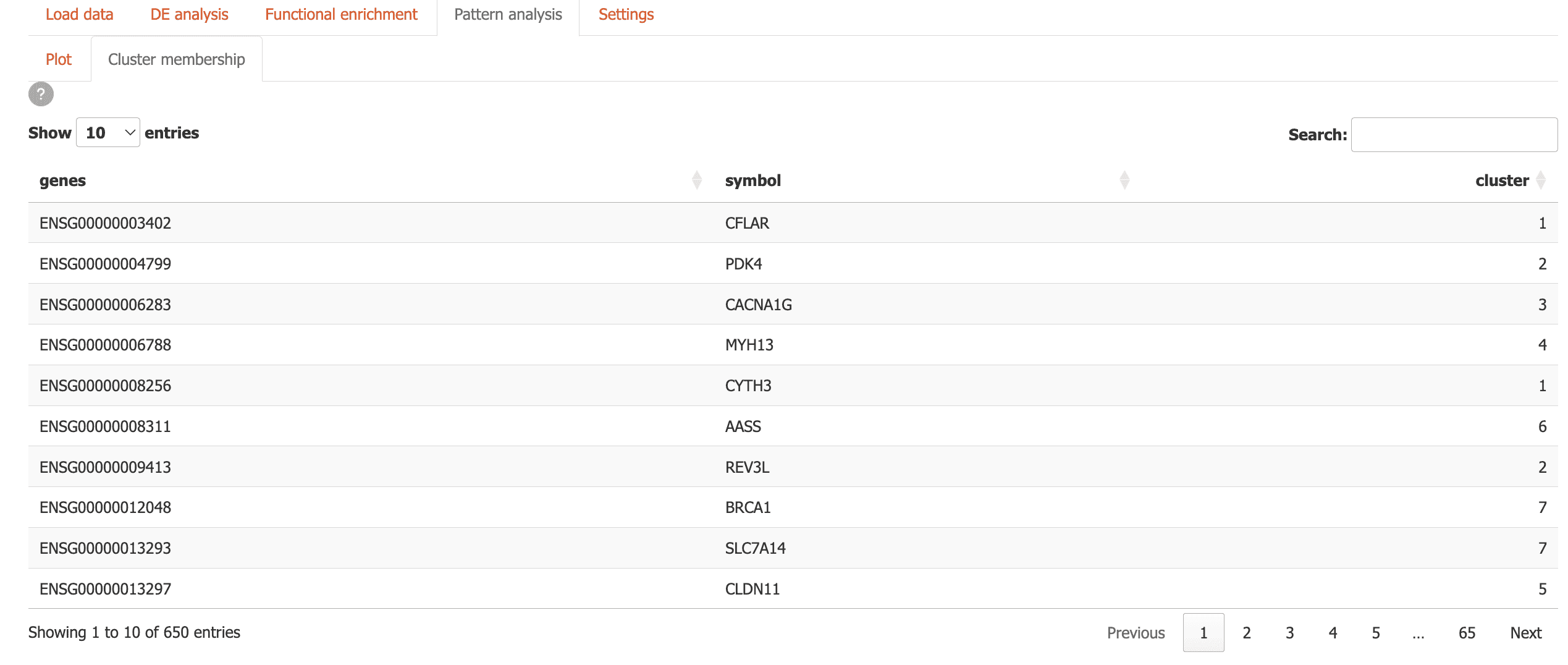
- Cluster Membership: Explore which genes belong to which clusters using an interactive table
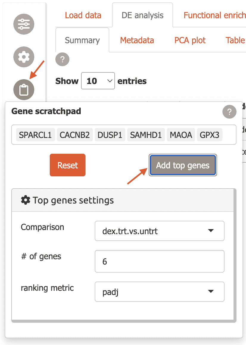
Gene scratchpad
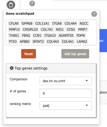
You can keep track of genes of interest across Carnation using the gene scratchpad.
To use this feature, click on the “Gene scratchpad” button in the sidebar.
-
To start you can add top differentially expressed genes from a specific comparison by using the “Top genes settings” and clicking “Add top genes”.
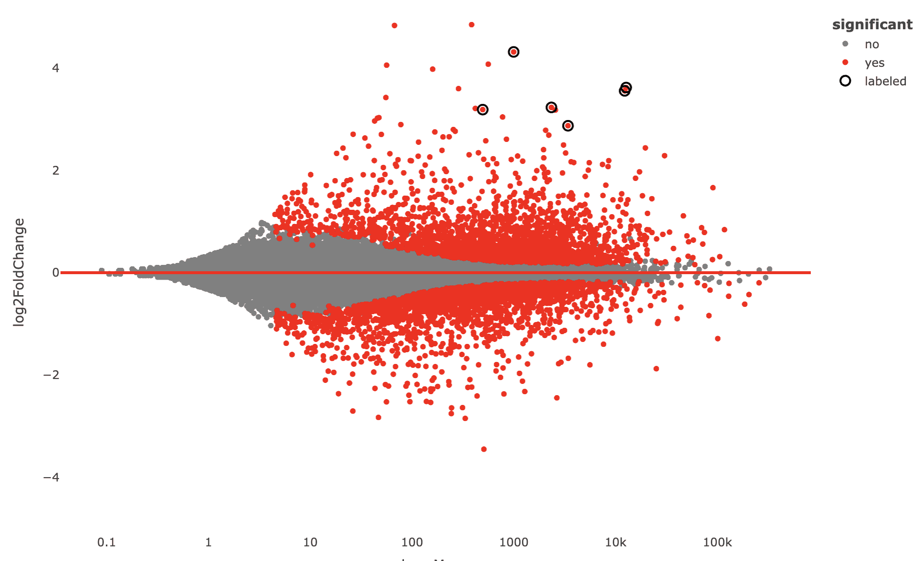
Now several plots in the “DE analysis” section will have these genes labeled, e.g. the MA plot, scatter plot, and others.
Labeled MA plot
Labeled scatter plot
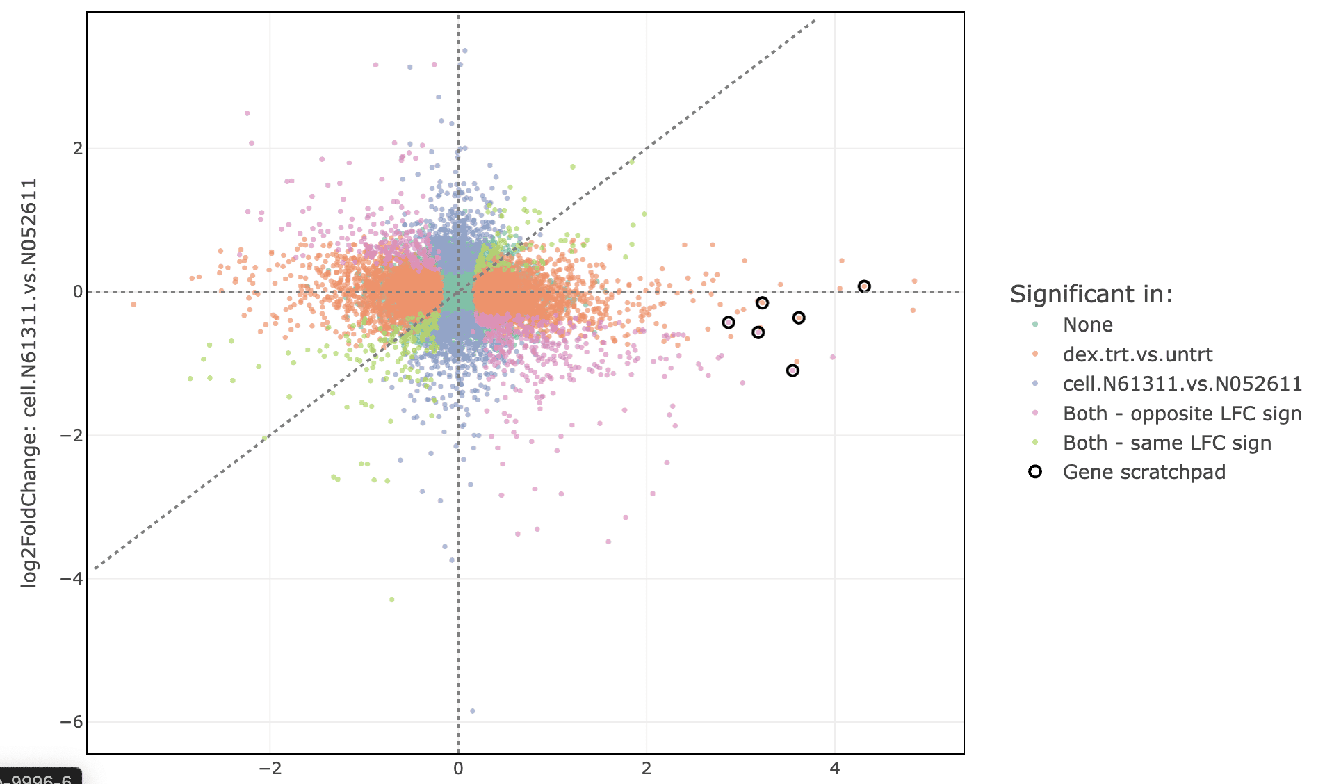
These genes can also be used to label the pattern analysis plot. Set “label” to “gene_scratchpad” and click “Refresh plot”.

Now the genes are labeled on the plot. You will also see a table below summarizing the clusters where these genes were found.

-
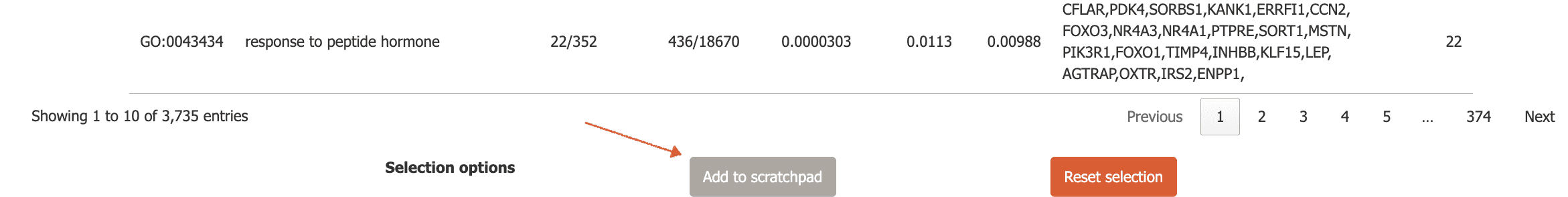
You can also quickly add genes to the scratchpad from functional enrichment tables
First, select your term of interest from the enrichment table
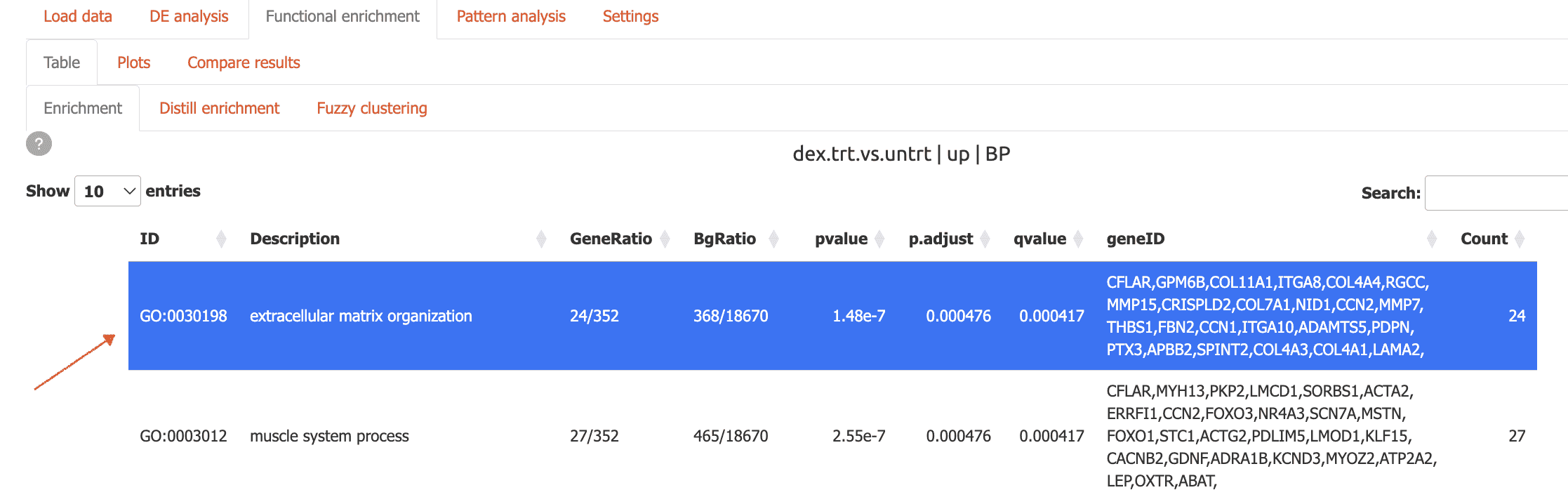
then, click the ‘Add to scratchpad’ button at the bottom of the page.
Now, these genes will be added to the scratchpad and can be used to label plots as shown above.
Server Mode
Carnation supports multi-user environments with authentication:
# Create user database
credentials <- data.frame(
  user = c('shinymanager'),
  password = c('12345'),
  admin = c(TRUE),
  stringsAsFactors = FALSE
)

# Initialize the database
shinymanager::create_db(
  credentials_data = credentials,
  sqlite_path = 'credentials.sqlite',
  passphrase = 'admin_passphrase'
)
Now run carnation with authentication
run_carnation(credentials='credentials.sqlite', passphrase='admin_passphrase')Summary
In summary, carnation adds to the rich Bioconductor
ecosystem providing a sophisticated interactive tool that makes it
easier to ask complex questions of the data and accelerate the process
of scientific discovery for biologists and computational scientists
alike. Other packages with comparable functionality include pcaExplorer
& iSEE.
However, carnation's unique combination of thoughtful
features, e.g. fuzzy search & gene scratchpad, in-built access
management system and deployment flexibility to single or multi-user
environments, makes it ideal as a platform for managing and sharing
complex bulk RNA-Seq projects with collaborators.
carnation currently supports the following widely-used
tools:
- Differential expression analysis: DESeq2, edgeR, limma
- Functional enrichment analysis: clusterProfiler (both overrepresentation & gene set enrichment analysis).
- Pattern analysis: DEGreport
The functional enrichment module incorporates plots from the GeneTonic and enrichplot packages.
Future plans include extending functionality to include support for other functional enrichment tools, e.g. topGO and coexpression analysis methods, e.g. WGCNA.
sessionInfo
sessionInfo()
#> R version 4.4.3 (2025-02-28)
#> Platform: x86_64-conda-linux-gnu
#> Running under: Ubuntu 24.04.4 LTS
#>
#> Matrix products: default
#> BLAS/LAPACK: /home/runner/work/carnation/env/lib/libopenblasp-r0.3.33.so;  LAPACK version 3.12.0
#>
#> locale:
#>  [1] LC_CTYPE=C.UTF-8       LC_NUMERIC=C           LC_TIME=C.UTF-8
#>  [4] LC_COLLATE=C.UTF-8     LC_MONETARY=C.UTF-8    LC_MESSAGES=C.UTF-8
#>  [7] LC_PAPER=C.UTF-8       LC_NAME=C              LC_ADDRESS=C
#> [10] LC_TELEPHONE=C         LC_MEASUREMENT=C.UTF-8 LC_IDENTIFICATION=C
#>
#> time zone: Etc/UTC
#> tzcode source: system (glibc)
#>
#> attached base packages:
#> [1] stats4    stats     graphics  grDevices utils     datasets  methods
#> [8] base
#>
#> other attached packages:
#>  [1] carnation_1.1.0             org.Hs.eg.db_3.20.0
#>  [3] AnnotationDbi_1.68.0        GeneTonic_3.0.0
#>  [5] dplyr_1.2.1                 DESeq2_1.46.0
#>  [7] airway_1.26.0               SummarizedExperiment_1.36.0
#>  [9] Biobase_2.66.0              GenomicRanges_1.58.0
#> [11] GenomeInfoDb_1.42.0         IRanges_2.40.0
#> [13] S4Vectors_0.44.0            BiocGenerics_0.52.0
#> [15] MatrixGenerics_1.18.0       matrixStats_1.5.0
#> [17] BiocStyle_2.34.0
#>
#> loaded via a namespace (and not attached):
#>   [1] fs_2.1.0                    bitops_1.0-9
#>   [3] enrichplot_1.26.1           webshot_0.5.5
#>   [5] httr_1.4.8                  RColorBrewer_1.1-3
#>   [7] doParallel_1.0.17           dynamicTreeCut_1.63-1
#>   [9] backports_1.5.1             tippy_0.1.0
#>  [11] tools_4.4.3                 R6_2.6.1
#>  [13] DT_0.34.0                   lazyeval_0.2.3
#>  [15] mgcv_1.9-4                  GetoptLong_1.1.1
#>  [17] withr_3.0.2                 prettyunits_1.2.0
#>  [19] gridExtra_2.3               cli_3.6.6
#>  [21] textshaping_1.0.5           logging_0.10-108
#>  [23] TSP_1.2.7                   sass_0.4.10
#>  [25] topGO_2.58.0                bs4Dash_2.3.5
#>  [27] S7_0.2.2                    askpass_1.2.1
#>  [29] ggridges_0.5.7              goseq_1.58.0
#>  [31] pkgdown_2.2.0               Rsamtools_2.22.0
#>  [33] systemfonts_1.3.2           yulab.utils_0.2.4
#>  [35] gson_0.1.0                  txdbmaker_1.2.0
#>  [37] DOSE_4.0.0                  R.utils_2.13.0
#>  [39] limma_3.62.1                RSQLite_3.52.0
#>  [41] visNetwork_2.1.4            generics_0.1.4
#>  [43] gridGraphics_0.5-1          shape_1.4.6.1
#>  [45] BiocIO_1.16.0               dendextend_1.19.1
#>  [47] GO.db_3.20.0                Matrix_1.7-5
#>  [49] abind_1.4-8                 R.methodsS3_1.8.2
#>  [51] lifecycle_1.0.5             edgeR_4.4.0
#>  [53] yaml_2.3.12                 qvalue_2.38.0
#>  [55] SparseArray_1.6.0           BiocFileCache_2.14.0
#>  [57] grid_4.4.3                  blob_1.3.0
#>  [59] promises_1.5.0              crayon_1.5.3
#>  [61] miniUI_0.1.2                ggtangle_0.1.2
#>  [63] lattice_0.22-9              billboarder_0.5.1
#>  [65] ComplexUpset_1.3.3          cowplot_1.2.0
#>  [67] GenomicFeatures_1.58.0      KEGGREST_1.46.0
#>  [69] pillar_1.11.1               knitr_1.51
#>  [71] ComplexHeatmap_2.22.0       fgsea_1.32.2
#>  [73] rjson_0.2.23                codetools_0.2-20
#>  [75] fastmatch_1.1-8             glue_1.8.1
#>  [77] ggfun_0.2.0                 data.table_1.17.8
#>  [79] vctrs_0.7.3                 png_0.1-9
#>  [81] treeio_1.30.0               gtable_0.3.6
#>  [83] assertthat_0.2.1            cachem_1.1.0
#>  [85] xfun_0.57                   S4Arrays_1.6.0
#>  [87] mime_0.13                   ConsensusClusterPlus_1.70.0
#>  [89] seriation_1.5.8             shinythemes_1.2.0
#>  [91] iterators_1.0.14            statmod_1.5.1
#>  [93] nlme_3.1-169                ggtree_3.14.0
#>  [95] bit64_4.8.0                 progress_1.2.3
#>  [97] filelock_1.0.3              rprojroot_2.1.1
#>  [99] bslib_0.10.0                otel_0.2.0
#> [101] colorspace_2.1-2            DBI_1.3.0
#> [103] mnormt_2.1.1                tidyselect_1.2.1
#> [105] bit_4.6.0                   compiler_4.4.3
#> [107] curl_7.1.0                  httr2_1.2.2
#> [109] graph_1.84.0                BiasedUrn_2.0.12
#> [111] SparseM_1.84-2              expm_1.0-0
#> [113] xml2_1.5.2                  ggdendro_0.2.0
#> [115] desc_1.4.3                  DelayedArray_0.32.0
#> [117] plotly_4.12.0               scrypt_0.1.6
#> [119] colourpicker_1.3.0          bookdown_0.46
#> [121] rtracklayer_1.66.0          scales_1.4.0
#> [123] psych_2.6.3                 mosdef_1.2.0
#> [125] rappdirs_0.3.4              stringr_1.6.0
#> [127] digest_0.6.39               shinyBS_0.65.0
#> [129] rmarkdown_2.31              ca_0.71.1
#> [131] XVector_0.46.0              htmltools_0.5.9
#> [133] pkgconfig_2.0.3             learnr_0.11.6
#> [135] dbplyr_2.5.2                fastmap_1.2.0
#> [137] rlang_1.2.0                 GlobalOptions_0.1.4
#> [139] htmlwidgets_1.6.4           UCSC.utils_1.2.0
#> [141] shiny_1.13.0                shinymanager_1.0.410
#> [143] farver_2.1.2                jquerylib_0.1.4
#> [145] jsonlite_2.0.0              BiocParallel_1.40.0
#> [147] GOSemSim_2.32.0             R.oo_1.27.1
#> [149] RCurl_1.98-1.18             magrittr_2.0.5
#> [151] GenomeInfoDbData_1.2.13     ggplotify_0.1.3
#> [153] patchwork_1.3.2             Rcpp_1.1.1-1.1
#> [155] reticulate_1.46.0           ape_5.8-1
#> [157] shinycssloaders_1.1.0       viridis_0.6.5
#> [159] stringi_1.8.7               rintrojs_0.3.4
#> [161] zlibbioc_1.52.0             MASS_7.3-65
#> [163] DEGreport_1.42.0            plyr_1.8.9
#> [165] parallel_4.4.3              ggrepel_0.9.8
#> [167] Biostrings_2.74.0           splines_4.4.3
#> [169] hms_1.1.4                   geneLenDataBase_1.42.0
#> [171] circlize_0.4.18             locfit_1.5-9.12
#> [173] igraph_2.3.1                reshape2_1.4.5
#> [175] biomaRt_2.62.0              XML_3.99-0.23
#> [177] evaluate_1.0.5              BiocManager_1.30.27
#> [179] foreach_1.5.2               tweenr_2.0.3
#> [181] httpuv_1.6.17               backbone_2.1.5
#> [183] openssl_2.4.0               tidyr_1.3.2
#> [185] purrr_1.2.2                 polyclip_1.10-7
#> [187] reshape_0.8.10              heatmaply_1.6.0
#> [189] clue_0.3-68                 ggplot2_3.5.2
#> [191] ggforce_0.5.0               broom_1.0.12
#> [193] xtable_1.8-8                restfulr_0.0.16
#> [195] tidytree_0.4.7              later_1.4.8
#> [197] viridisLite_0.4.3           ragg_1.5.2
#> [199] tibble_3.3.1                clusterProfiler_4.14.0
#> [201] aplot_0.2.9                 registry_0.5-1
#> [203] memoise_2.0.1               GenomicAlignments_1.42.0
#> [205] cluster_2.1.8.2             sortable_0.5.0
#> [207] shinyWidgets_0.9.1          shinyAce_0.4.4